Flashy demos of robotic systems are popping up on our feeds almost every day, showing robots that can build boxes, clean offices, and do household tasks. But we typically don’t know how these systems were actually built and trained, and in some cases whether it’s really the robot operating or a teleoperator behind the scenes.
How does a field collaboratively learn to build better and more trustworthy robots if most systems are shrouded in mystery?
To change this, we trained a robot on a challenging but highly requested task: cloth folding. We built and trained a bimanual robot that achieves 90% success rate on folding a random t-shirt.
Autonomous folding of crumpled t-shirts (Level 2)
To get there we used 8 bimanual robot setups, spent ~131 hours collecting demonstrations, and used 5,000+ GPU hours across dozens of training runs. And to lift the veil on building end-to-end realistic robotic use cases, this blog walks through every step:
- Hardware: which robot, cameras, and teleop system to use
- Data collection: how to collect and filter high-quality demonstrations
- Training recipes: which model architecture and hyperparameters work
- Experiments: careful ablations to improve the overall pipeline
- Evaluation: what metrics give good signal and are reliable enough
- Takeaways: what we learned and what we’d do differently next time
This post aims to serve as a blueprint for building real-world robotic learning systems with current open-source tools. Whether you are in industry, research, or your garage, this guide will help you move beyond simple toy projects.
This project was made possible entirely by LeRobot. Everything discussed in this blog is available in LeRobot v0.5.1 and ready for the community to use.
All resources from this project are open-source:
So we want to build a robot to fold clothes, but what kind of robot should we use? A humanoid? A single arm? Or something else? Let’s have a look at the design choices around the hardware.
Hardware
LeRobot handles the software stack, but you still need the physical hardware. Below we cover the base robot, custom grippers, a cheap 3D-printed teleop setup that outperformed the expensive one, and the camera layout.
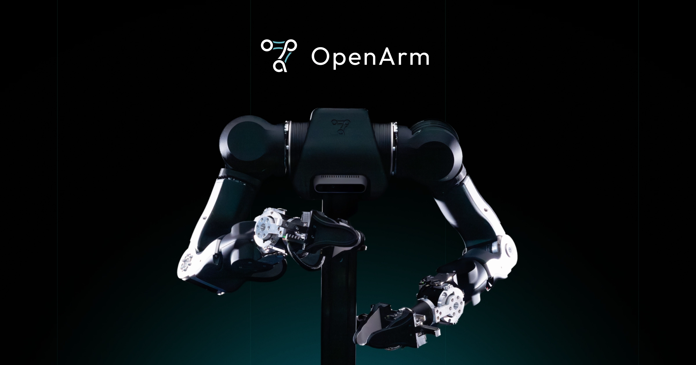
The Robot: Bimanual OpenArm
For starters, the robot. We used the bimanual OpenArm. These are open-source, human-like robot arms developed by Enactic and sold by multiple vendors like WowRobo. Two reasons drove this choice:
- Smaller teleop gap. When the robot’s kinematics match a human arm, the teleoperator’s motions transfer more naturally, meaning less mental remapping and faster learning. The humanoid form factor also aligns with where the ecosystem is heading: more human-form robots means more transferable data.
- Open source, good specs. Solid payload, good reach, and fully open hardware. We extended the upper arm (the bicep segment) by +5 cm to increase reach since our setup doesn’t have a hip or torso to provide additional workspace.
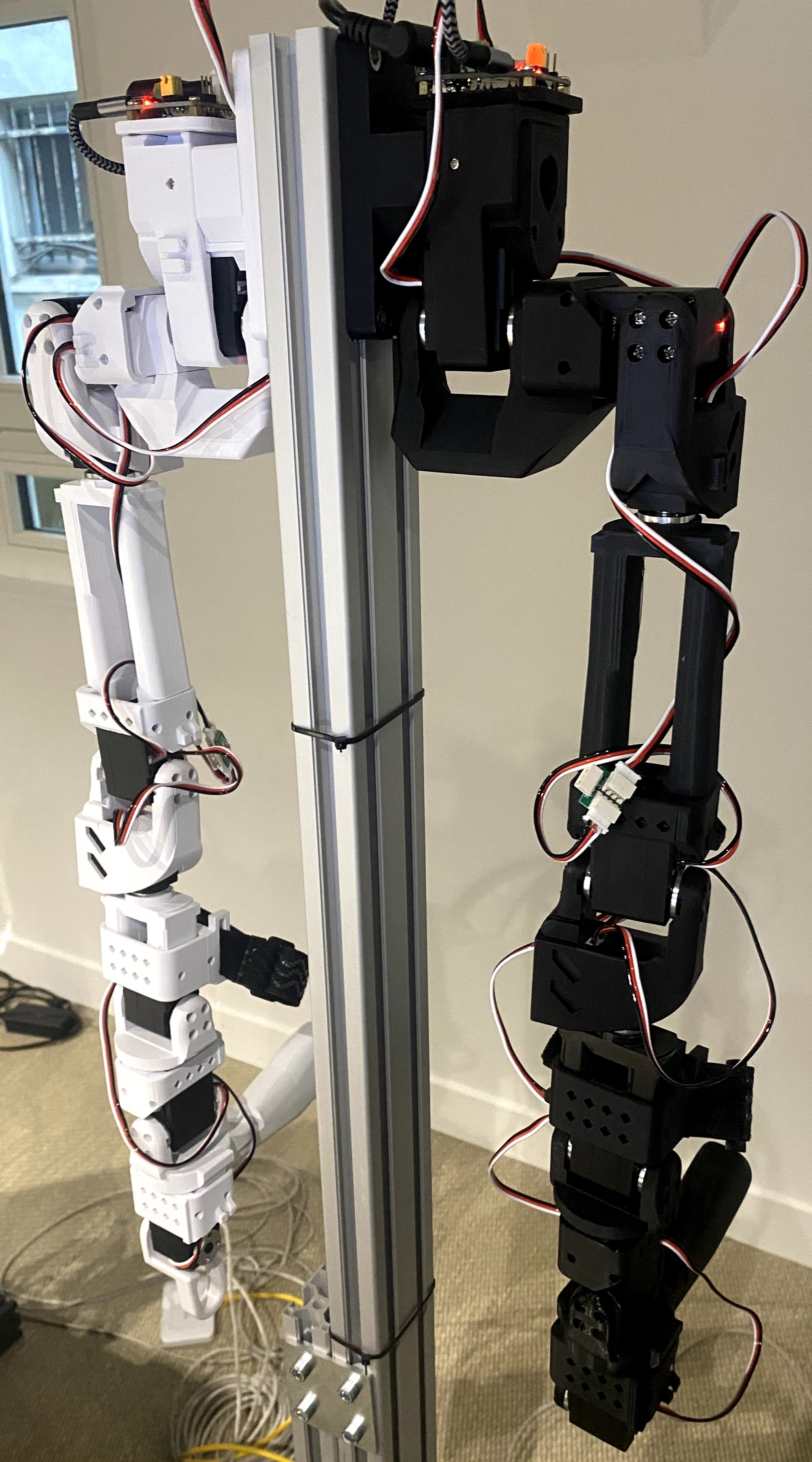
Everything is mounted on aluminum extrusion profiles, which let us quickly iterate on the physical arrangement and adjust both teleop and robot height between sessions to increase data diversity. We also designed custom grippers with a larger surface area, giving the robot a broader contact patch to grip, pinch, and slide fabric reliably. All custom hardware modifications (extended bicep, gripper jaws, covers) are available.
Teleop Arms: OpenArm Mini
Next, we need a way to control the robot. We started with full-size OpenArm as leader arms for teleoperation. They seemed like the natural choice: same kinematics as the follower arms, one-to-one mapping.
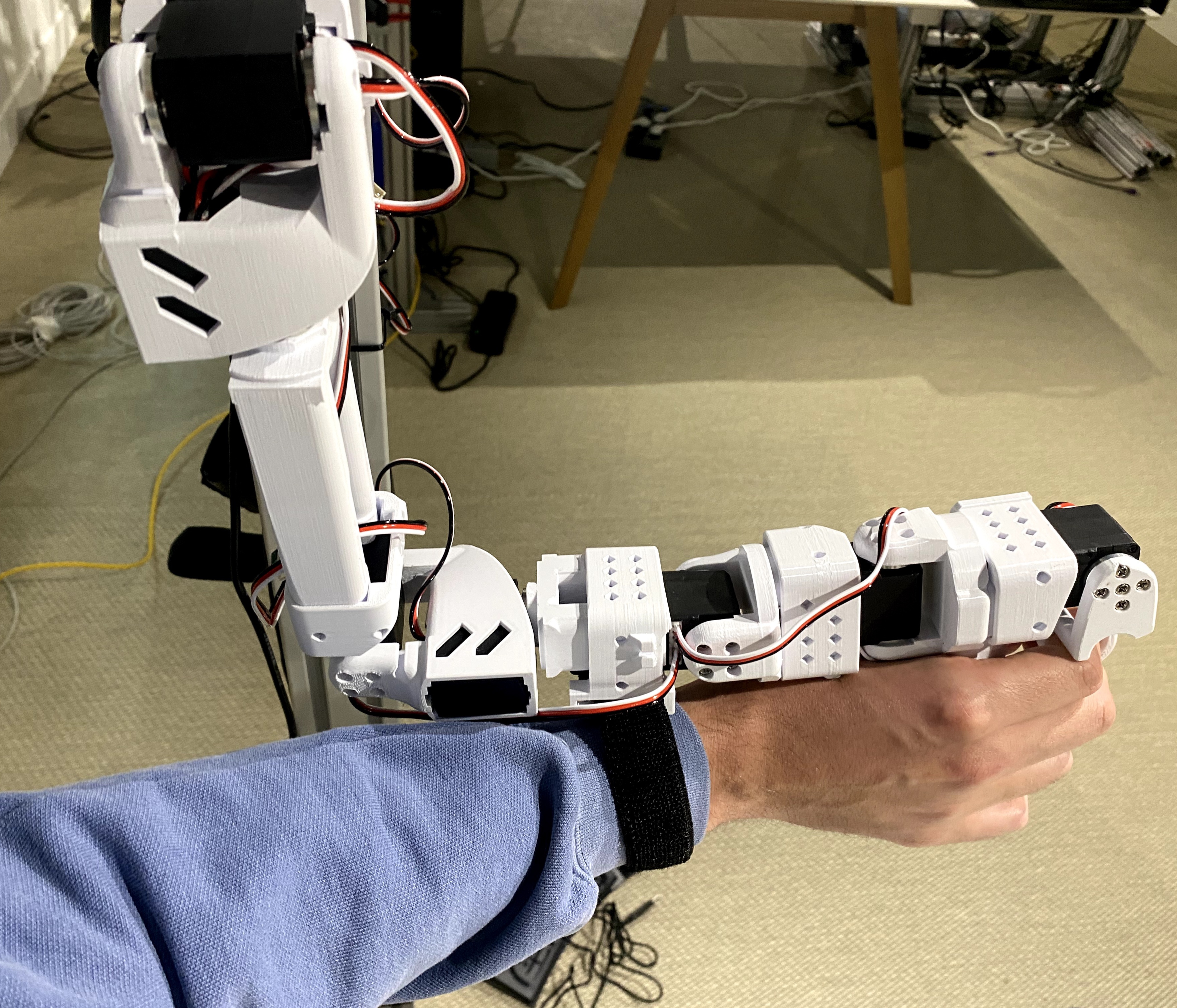
However, we quickly realized we needed a teleoperator arm with less inertia, that allows for fast and precise manipulation, and more adaptability to different human morphologies. This led us to experiment with friction and gravity compensation - which improved the operator’s experience, but ultimately we decided to develop the OpenArm Mini: small, Feetech-based, 3D-printed leader arms based on the SO-101 design. These gave us:
- Less inertia for quicker and more deliberate motions that cloth folding demands
- Arm-length agnostic and adaptable to any human operator size
- Incredibly cheap (~120 EUR per arm) making it easy to scale to multiple stations
- Still supports itself: strong enough to move during human-in-the-loop corrective data collection
One small detail mattered more than expected: the wrist strap. It locks the operator’s wrist to the leader arm, providing rotational control essential for precise manipulation.
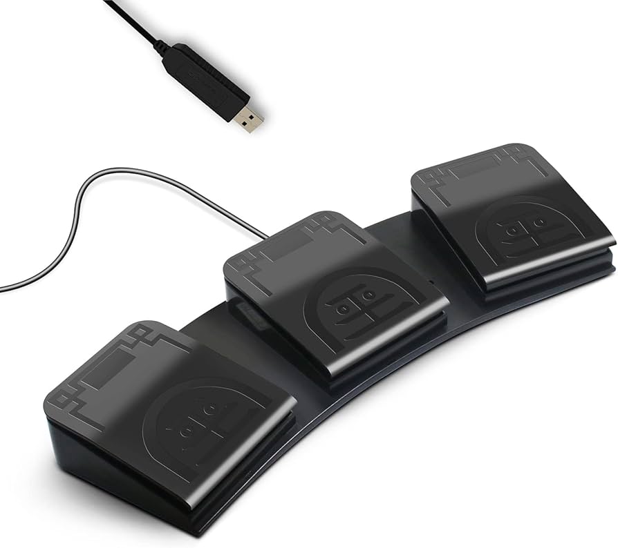
Another feature that made a surprisingly big difference: when both your hands are on the leader arms, you need a hands-free way to start and stop episode recording. USB foot pedals solved this elegantly.
Sensors
We use three cameras, each serving a purpose. The base camera is mounted between the arms and provides a wide-angle overview of the full workspace, the model’s primary understanding of the task state. The two wrist cameras are mounted directly on the end-effectors. Because they move with the grippers, they provide a natural depth signal and give a close-up view for precise manipulation. They also act as a proxy for touch, being so close to the grippers, they capture contact details: grip quality, slip, that humans normally sense through their fingers. More details about the resolution and FPS of each later on. While additional cameras could help, every extra image stream requires more compute and time to process; three was the tradeoff we settled on.
Camera links: Base camera (Fafeicy OV2710) / Wrist cameras (Arducam IMX708)
Beyond RGB cameras, the only other sensor data we used were the joint encoders from the arm’s motors. No torque sensors, no force/touch sensing, no audio, no IMUs, no depth cameras. All the results in this blog were achieved with just camera images and joint positions. While additional sensing modalities could potentially improve performance, the overhead of integrating, calibrating, and maintaining extra sensors adds real engineering complexity. Given how well this minimal setup performed, it’s hard to argue the tradeoff is worth it for this application.
LeRobot Integration
Besides integrating the OpenArm robot into LeRobot, we needed two additional pieces of infrastructure: a low-level driver and an operator-friendly interface.
On the driver side, we added CAN-bus support. CAN-bus is the communication protocol the arm’s motors use. Think of it as a shared wire where LeRobot sends position commands (“move joint 3 to 45°”) and reads back the current joint angles.
On the operator side, we built a recording UI so non-technical operators can start, stop, and review episodes without touching the CLI. With 8 setups running in parallel, having a simple interface that anyone on the team could use without training was essential for keeping data collection moving.
With the hardware in place, the next step was the hardest and most time-consuming part of the entire project: collecting good data. And “good” is much harder to define than it sounds.
Data Collection
Data collection was the longest phase of this project, and arguably the most important. No amount of compute can compensate for bad demonstrations.
T-shirt folding involves deformable objects with complex contact dynamics: simulation can’t faithfully reproduce how fabric crumples and slides, world models can’t yet predict cloth deformation reliably, and RL from scratch on real hardware is too sample-inefficient for a task this long-horizon (though RL on top of a pretrained VLA is a promising future direction). That leaves real-world teleoperation as the practical path. We chose leader-follower arms because they match the robot’s kinematics exactly (what the operator does is what the robot does), giving low latency, high precision, and support for DAgger, where the teleop setup takes over from a running policy to collect corrections.
We ran 8 setups in parallel, optimizing for maximum diversity: 25+ different t-shirts, 8 different backgrounds, and varying camera and robot heights between sessions. We structured collection into two task levels: Level 1 (fold a laid-out shirt) and Level 2 (spread a messy shirt, fold it, place it aside).
We never strongly controlled lighting conditions during data collection or evaluation. The only requirement was having enough light for the cameras. All work happened in an open coworking space throughout different times of day: sometimes daylight, sometimes artificial light at night, sometimes a mix. No special lighting rigs, no effort to homogenize conditions across episodes or rollouts.
Learning to Teleoperate
Here’s an honest truth: early data collection is worse than the final data. Teleoperating a bimanual robot is a genuine skill, and it takes practice. The first episodes are slow, not deliberate, and full of failed attempts. Over hours of practice, operators get dramatically better, with smoother motions, faster execution, and more consistent grasps.
This raises an important practical question: when do we start using the robot operators’ data? Every hour of data collection requires a human operator, it’s expensive and doesn’t scale easily. But bad demonstrations aren’t just wasted effort, they might actively hurt the model, which can reproduce hesitations and inconsistent strategies. But defining what makes a “good” demonstration is itself an unsolved problem in robot learning. Duration is a rough proxy, a fast episode can still contain poor grasps, and a slow one can be perfectly executed. We ended up relying on a combination of heuristics and a learned reward model (introduced later) to separate useful data from harmful data.
Aligning on a common strategy across operators was equally important. Folding is a very multi-modal task (there are many valid ways to fold a t-shirt) and with unlimited data per approach the model could probably learn them all. But at our scale, mixing strategies means each one is under-represented. Aligning on a single strategy is a more data-efficient path. Before each recording sprint, we held brief alignment sessions: experimenting with different techniques, sharing our learnings and then converging on the most efficient fold sequence.
Tips for Good Data Collection
After weeks of collecting data across operators, these are the guidelines we found most useful:
- Practice before you record. Consistent, deliberate demonstrations are more valuable than hesitant or inconsistent ones.
- Quality over speed. High-quality task execution is more valuable than fast, sloppy ones.
- Be consistent within episodes. The model learns a coherent strategy more easily than movements that vary wildly each time.
- Start small, then extend. Train a quick model, see what fails, then add diversity. Don’t try to collect the perfect dataset on day one.
- Speed after quality. Once you’ve dialed in quality and a consistent strategy, optimize for speed. But never sacrifice quality for it.
- Watch your setup, not just your data. If the rig vibrates or frustrates operators, fix that before collecting more.
What we ended up with
After multiple weeks of collection across 8 setups, we had 5,688 episodes, the full dataset. Those ~131 hours of recorded demonstrations represent a fraction of the total time operators spent on the project, which also included practicing teleoperation, setting up and repairing robots, and aligning on strategies between sessions. This shows that data collection is a lot more than just recording demonstrations, and being very efficient with your time is key. Not all episodes are equally useful either: some contain hesitations, inconsistent strategies, or poor fold quality. Later in the project, we built a smaller high-quality dataset of 1,200 episodes by selecting the best recordings from the full set and adding new demonstrations collected with a more unified strategy.
| Metric | Full dataset | High-quality dataset |
|---|---|---|
| Total episodes | 5,688 | 1,200 |
| Total frames | 14.1M | 3.2M |
| Total hours | ~131 h | ~30 h |
| FPS | 30 | 30 |
| Cameras | 3 (base 480×640, wrists 720×1280) | 3 (same) |
| Action dims | 16 (7 joints + gripper × 2 arms) | 16 (same) |
All data is stored in the LeRobotDataset v3.0 format, which encodes camera streams as video rather than individual images. This makes the dataset 20x–40x more compressed compared to storing raw frames, making it practical to share and stream datasets of this scale.
The grid below shows one frame from each of 100 different episodes. Notice the variation in t-shirt color, background and camera viewpoint.
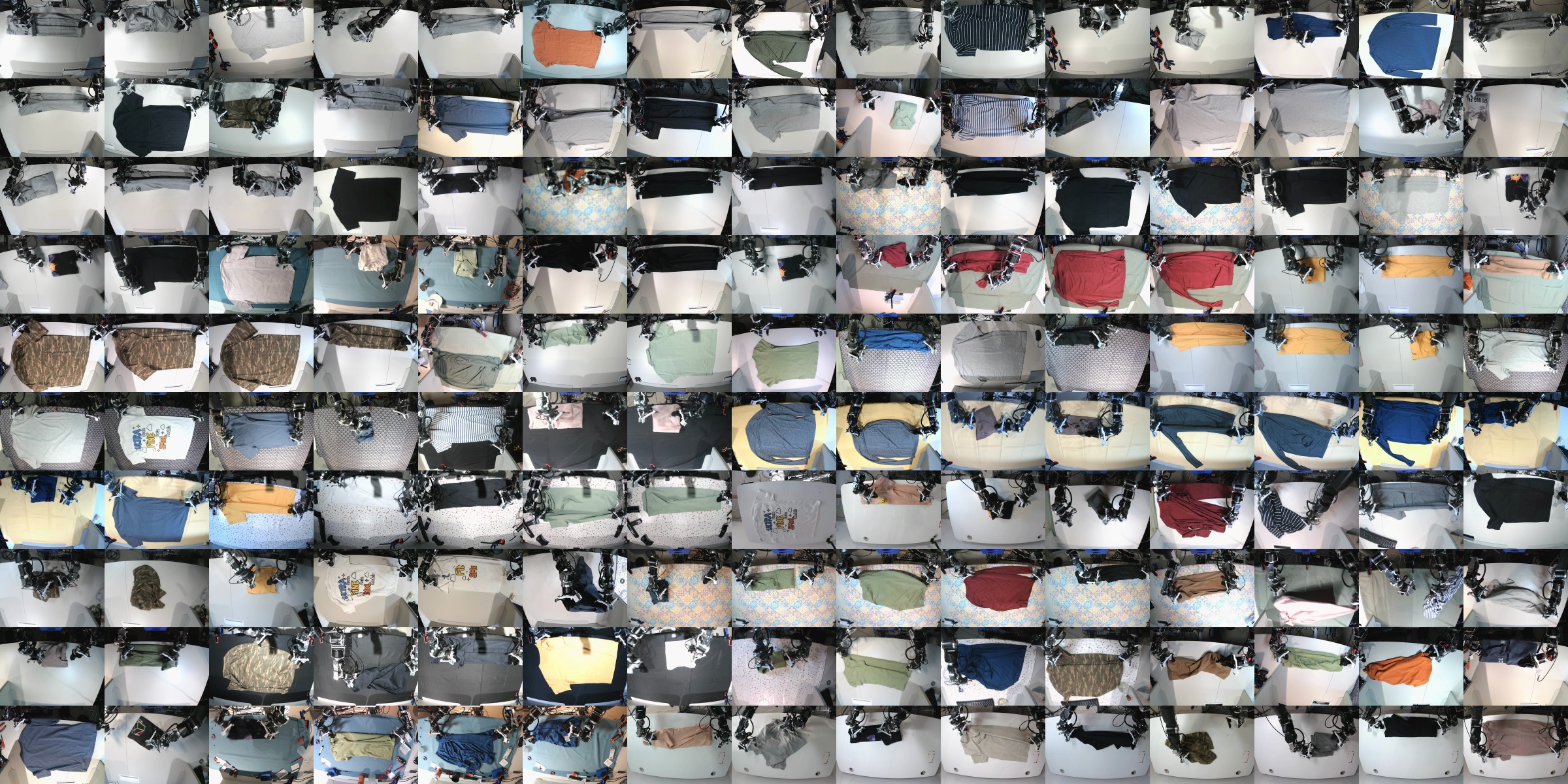
Explore the dataset yourself with the LeRobot Data Visualizer:
Model and Evaluation Setup
Before diving into experiments, let’s establish the model we’re training and how we measure performance. These stay constant across every iteration.
Model Architecture
The dominant approach in robot learning today is to train a Vision-Language-Action (VLA) model: a single neural network that takes in camera images and a task description and outputs motor commands. The recipe most labs follow is to pretrain a VLA on large, multi-robot, multi-task datasets to learn general visual and manipulation priors, then fine-tune it on data from your specific robot and task. Several strong pretrained VLAs exist: π0, π0.5, GR00T, SmolVLA, among others. We chose to use π0 and π0.5 because they showed the strongest performance in our early experiments, likely due to the scale of their pretraining data. We start from the pretrained checkpoints and fine-tune on our folding data.
The model takes in three things: camera images (3 views: base + 2 wrist), joint angles (16D: 7 joints + gripper per arm), and a language prompt (“fold the t-shirt”). The images pass through a frozen SigLIP vision encoder that converts raw pixels into visual tokens, a compact representation the rest of the model can work with. Those visual tokens, the text, and the joint state all feed into the Gemma VLM backbone (2B parameters), which fuses the three modalities through cross-attention. This is where the model builds its understanding of the scene: what the shirt looks like, where the arms are, and what it’s supposed to do. The backbone’s output then conditions the Action Expert (300M parameters), which uses flow matching to turn random Gaussian noise into a coherent sequence of 30 actions, which equals one second of joint targets and gripper commands. Flow matching lets the model represent multi-modal action distributions: when there are multiple valid ways to grasp a sleeve, it can capture that ambiguity rather than averaging to a meaningless middle ground.
Real-Time Chunking (RTC)
The model outputs 30 actions at once (a “chunk”), but generating that chunk takes ~100–200ms, during which the robot is still moving. Without RTC, the robot would pause between chunks while waiting for the next prediction, producing jerky stop-and-go motion. RTC solves this by generating the next chunk while the current one is still executing. The key idea: by the time the new chunk is ready, several actions from the old chunk have already been executed and can’t be changed, so RTC freezes those committed actions and inpaints the rest of the new chunk to be consistent with them. This produces smooth, continuous motion with no pauses.
In practice, RTC sped up our rollouts by at least a factor of 2 compared to synchronous inference.
All experiments use RTC with an action queue size of 30 and a maximum action horizon of 20, along with action interpolation (upsampling from 30 Hz to 90 Hz) which makes the robot much quieter and smoother.
Training recipe
We fine-tune two variants of this architecture: π0, the base flow-matching VLA, and π0.5, an improved version with more pretraining data and refinements to the denoising process. Both start from pretrained checkpoints. Training runs on 8× H100 GPUs with a per-GPU batch size of 32 (a total batch size of 256), gradient accumulation, and using AdamW with a learning rate of 1e-4 (warmup + cosine decay). The large batch size is important for stable VLA training, and it’s what drives the multi-GPU requirement.
With ~131 hours of video-encoded demonstrations, keeping data close to compute matters. Hugging Face Storage Buckets now make this straightforward: they provide S3-like object storage with a built-in CDN that can be pre-warmed in your training region, and Xet deduplication means re-uploading a slightly modified dataset only transfers the diff. Datasets stored on the Hub or in buckets can be streamed directly to GPUs with no extra infrastructure.
Evaluation Protocol
Evaluation is as hard as training. In robotics and with real hardware, no standardized benchmarks exist. If your evaluation protocol is inconsistent, every downstream decision will be wrong.
For every experiment, we evaluate the model on:
- 5 different t-shirts for Level 1 (laid-out to fold)
- 5 different t-shirts for Level 2 (messy to spread to fold, then place aside)
Each t-shirt fold is attempted twice consecutively, giving 10 rollouts per level and 20 rollouts total per experiment. Every evaluation is filmed and scored from video afterward, so judgment is decoupled from execution.
The evaluation protocol (t-shirts, attempts count, scoring rubric, and filming setup) is identical across every experiment.
Metrics
We report four complementary metrics:
- Success Rate. Binary pass/fail per rollout.
- Score. Partial credit based on subtasks completed. This distinguishes a model that consistently reaches Fold 3 from one that fails at Unfold, even if neither achieves full success.
Scoring rubric Level 1 and Level 2
Level 1 Laid-out shirt to fold (shirt starts flat):
| Subtask | Points |
|---|---|
| Do first horizontal fold | +10 |
| Do second horizontal fold | +10 |
| Do third vertical fold | +10 |
| Do final fold | +10 |
| Rotate | +10 |
| Maximum per rollout | 50 |
Level 2 Messy shirt to spread, fold, and place aside:
| Subtask | Points |
|---|---|
| Unfold (spread the shirt) | +50 |
| Fold 1 | +10 |
| Fold 2 | +10 |
| Fold 3 | +10 |
| Fold 4 | +10 |
| Rotation + Place aside | +10 |
| Maximum per rollout | 100 |
Scores are summed across all the rollouts in an experiment. With 10 Level 1 rollouts (max 50 points each) and 10 Level 2 rollouts (max 100 points each), the maximum total score per experiment is 1,500 points.
- Fold quality. A 1–5 rating of the final fold appearance, averaged across successful rollouts.
- Completion time. Seconds to complete Level 1/Level 2, averaged across successful rollouts.
Statistical uncertainty
With 20 rollouts per experiment, even large apparent differences can be statistically indistinguishable. We report Clopper-Pearson 90% confidence intervals on all success rates and run formal pairwise significance tests using STEP (Snyder et al., 2025). Running 50-100 rollouts per experiment would give tighter estimates but was not feasible for us across 11 experiments on real hardware.
From Data to Deployment
With the data collected, hardware running, and evaluation protocol fixed, we began training. What follows is the chronological story of how we iterated from a barely-working baseline to a 90% success rate, and what we learned at each step.
First attempt: training on all data
We started with the simplest possible recipe: train π0 and π0.5 on the full dataset of 5,688 episodes for 200k steps each (taking around 27 hours in our case).
| Experiment | Model | Data | Steps | Key change |
|---|---|---|---|---|
| 1.1 | π0 | All data (5,688 episodes) | 200k | Baseline |
| 1.2 | π0.5 | All data (5,688 episodes) | 200k | Baseline |
When we evaluated, the results were mixed. Experiment 1.1 (π0) achieved 40% total success rate (80% Level 1) but 0% Level 2. Experiment 1.2 (π0.5) managed only 20% total (40% Level 1), also with 0% Level 2. The models could sometimes fold a laid-out shirt, but they were slow and produced poor-quality folds. Level 2 (spreading a messy shirt before folding) was completely out of reach.
Watching the rollouts, we suspected that the problem was in the data. Different operators used different grip points and strategies for unspreading the shirt, and the diversity in our dataset was high. The model didn’t converge enough and was producing indecisive motions.
An additional early lesson: undertraining makes the policy shaky. Make sure your model has converged before drawing conclusions about what works.
Improving the data
Before adding algorithmic complexity, we addressed the data quality problem directly.
Filtering
We filtered episodes in two ways:
- End-state image filtering to discard episodes where the final frame doesn’t show a properly folded shirt. If the end result isn’t good, the demonstration isn’t useful.
- Length-based filtering using the LeRobot data visualizer to remove outliers. Episodes that are suspiciously short tend to be low quality.
Stage-Aware Reward Modeling (SARM)
To go beyond binary keep/discard filtering, we trained a reward model: SARM (Stage-Aware Reward Modeling). The core problem SARM solves: how do you measure “progress” in a long, multi-stage task like t-shirt folding, where demonstrations vary wildly in length and strategy? You can’t just use elapsed time, a shirt that’s fully flattened might happen at frame 200 in one demo and frame 800 in another. SARM instead learns a semantic notion of progress that generalizes across demonstrations.
How it works. SARM is a vision-language reward model built on a frozen CLIP backbone. It takes 8 RGB frames (sampled 1 second apart from the base camera), a task description (“fold the t-shirt”), and the robot’s joint state. The language conditioning means the same model could in principle score different tasks; it’s not hard-coded to folding.
The images and text are encoded by CLIP into embeddings. These flow into a Stage Transformer, which classifies which subtask the robot is in (e.g., “grab”, “flatten”, “fold”, “place”), and a Subtask Transformer, conditioned on the predicted stage, which estimates fine-grained progress τ within that stage. The final output is a single progress score (stage + τ, normalized to [0, 1]). This two-level decomposition makes the reward signal stable across demonstrations of different lengths and styles: a fully flattened shirt always maps to roughly the same progress value, regardless of how long it took to get there. The score is used downstream for data curation (ranking episodes by quality) and RABC training weights (emphasizing high-progress actions during policy training).
Training data. SARM supports multi-stage annotations, but we use it in single-stage mode: the entire task (Level 2, which includes Level 1) is treated as one stage with progress going linearly from 0 to 1. This means no human subtask annotation is needed, progress labels are derived directly from the frame index within each episode.
Once trained, SARM can score any trajectory, including noisy demonstrations it was never trained on. It predicts a 0–1 progression signal at every timestep, correctly identifying mistakes (drops in value) and progress (increases) in real time:

We annotated every episode in both datasets using SARM. This gave us continuous per-timestep quality scores that we could use in two ways: for data curation (scoring and ranking episodes) and for reward-weighted training (which we introduce next).
Better training recipes
With cleaner data and SARM scores in hand, we turned to how the model trains on that data.
Relative actions
Following the UMI approach, we switched from absolute actions to relative action trajectories: each action in the chunk is an offset from the robot’s current state at prediction time, not from the previous action. The state observation remains absolute; only the action targets are relative. This avoids error accumulation (unlike true delta).
See the LeRobot action representations docs for a full guide.
The result: experiment 1.3 (π0.5 + relative actions) jumped to 35% total success rate and 70% Level 1, up from 1.2’s 20% total and 40% Level 1.
RABC (Reward-Advantage-Based Conditioning)
Next, we put SARM’s per-timestep scores to work during training with RABC (Reward-Aligned Behavior Cloning). Standard behavior cloning treats every action in the dataset equally. RABC instead computes a per-timestep “progress delta” from SARM (the change in predicted task progress over one action chunk) and uses it to weight the training loss. A threshold κ controls how selective the weighting is: actions with progress above κ get full weight, those below are softly down-weighted, and negative-progress actions are clipped to zero weight entirely. The result is that the policy focuses on the best moments in each demonstration without discarding entire episodes.
Combining everything
Experiment 1.7 combined relative actions + RABC. The result: 40% total success rate, 80% Level 1, the best of initial training.
| Experiment | Key change | Total SR | Level 1 SR | Level 2 SR |
|---|---|---|---|---|
| 1.1 | π0 baseline | 40% | 80% | 0% |
| 1.2 | π0.5 baseline | 20% | 40% | 0% |
| 1.3 | π0.5 + Relative actions | 35% (+15) | 70% (+30) | 0% (+0) |
| 1.7 | π0.5 + Relative + RABC | 40% (+20) | 80% (+40) | 0% (+0) |
The trend was encouraging, but one number was impossible to ignore: every initial-training experiment achieved exactly 0% Level 2 success. Algorithmic improvements alone couldn’t compensate for the inconsistency in the full dataset.
DAgger: targeted corrections
Throughout our work on Level 1, we developed and integrated DAgger (Dataset Aggregation) as a Human-in-the-Loop (HIL) data collection method in LeRobot. The idea: the operator watches the policy run, pauses when it fails, teleoperates a recovery, and hands control back. This generates correction data precisely where the model struggles. We add both the autonomous segments (where the policy acted on its own) and the human corrections back into the training dataset.
We didn’t test DAgger in an isolated experiment, but added the correction data to both the full dataset and the high-quality dataset. In our early experiments, using DAgger to collect targeted corrections proved very beneficial for making the policy more robust to failures; the model learns to recover from states it would otherwise get stuck in. The full Human-in-the-Loop infrastructure is now merged into LeRobot for anyone to use.
The breakthrough: high-quality data
No initial-training experiment cracked Level 2. We needed a fundamentally better dataset.
We went back to data collection with a clear plan: collect new demonstrations, with a more unified strategy across operators. Every episode followed similar grip points, sequences, and timing. We also manually curated the best episodes from the large dataset, selecting only those with consistent technique and clear progress.
The result was the high-quality dataset: 1,200 episodes combining the best of the original data with new, strategically collected demonstrations.
We then fine-tuned the best initial-training checkpoints on this curated dataset for 100k steps:
| Experiment | Base | Key change | Total SR | Level 1 SR | Level 2 SR |
|---|---|---|---|---|---|
| 2.1 | 1.3 | HQ data only | 40% (+5) | 70% (+0) | 10% (+10) |
| 2.2 | 1.3 | HQ + RABC + Relative | 75% (+40) | 100% (+30) | 50% (+50) |
| 2.5 | 1.7 | HQ + RABC + Relative | 90% (+50) | 100% (+20) | 80% (+80) |
The jump was dramatic. Experiment 2.5 reached 90% total success rate: 100% Level 1, 80% Level 2, up from 40% with initial training. The same architecture, the same training recipe, just better data and more fine-tuning.
Both 2.2 and 2.5 used the same recipe (HQ + RABC + Relative Actions), but 2.5 fine-tuned from 1.7 (the stronger base with relative actions + RABC already baked in) while 2.2 fine-tuned from 1.3. The difference (75% → 90%) likely reflects this stronger starting point. Data quality was the single biggest lever, and RABC’s effect was strongest on Level 2, the longer, harder task where emphasizing the best demonstrations mattered most.
Here is an uncut Level 1 evaluation run from Experiment 2.5, 15 minutes of continuous folding, no human intervention:
Autonomous folding from flat state (Level 1)
We evaluate on two difficulty levels. Level 1 starts from a laid-out t-shirt; Level 2 starts from a crumpled mess and requires spreading, folding, and placing the shirt aside. Results are from our best model (Experiment 2.5), evaluated over 20 rollouts:
| Task | Success Rate | Avg. Completion Time |
|---|---|---|
| Level 1 Laid-out to Fold | 100% | 40.8 s |
| Level 2 Messy to Spread to Fold to Place aside | 80% | 95.9 s |
| Combined (Total SR) | 90% |
What didn’t work
Not every idea improved results:
- RABC on the full dataset (experiments 1.4, 1.5; without relative actions): we applied SARM’s reward weighting directly during initial training on the full dataset, with different selectivity thresholds. Both performed worse than the baseline (1.4: 15% total, 1.5: 0% total). The reward model was only trained on the high-quality dataset, so when applied to the larger dataset it likely down-weighted too much Level 1 data, meaning the model couldn’t reliably accomplish the first steps of the task.
- Mirroring augmentation (experiment 2.3): only 5% total success rate. Mirroring the data doubles the number of valid strategies the model sees, which is the opposite of what we needed: convergence on a single consistent approach.
- Larger chunk size (experiment 2.4, chunk=45): no improvement over the default chunk size of 30.
Full comparison
Now that the full journey is clear, here is the complete picture across all 11 experiments.
| # | Model | Data | Steps | Key change |
|---|---|---|---|---|
| 1.1 | π0 | All | 200k | Baseline |
| 1.2 | π0.5 | All | 200k | Baseline |
| 1.3 | π0.5 | All | 200k | Relative actions |
| 1.4 | π0.5 | All | 200k | RABC κ=0.01 |
| 1.5 | π0.5 | All | 200k | RABC κ=0.0215 |
| 1.7 | π0.5 | All | 200k | Rel + RABC κ=0.0215 |
| 2.1 | π0.5 | HQ | 100k | From 1.3 |
| 2.2 | π0.5 | HQ | 100k | From 1.3 + RABC + Rel |
| 2.3 | π0.5 | HQ + mirror | 100k | From 1.3 + Rel + mirroring |
| 2.4 | π0.5 | HQ | 100k | From 1.3 · chunk=45 |
| 2.5 | π0.5 | HQ | 100k | From 1.7 + RABC + Rel |
Total score captures partial progress that binary success rate misses: even failed rollouts earn credit for completed subtasks. The CLD letters (from STEP sequential testing with Bonferroni correction, α = 0.10, per-pair α < 0.0018, nmax = 50, following the Toyota Research Institute (TRI) statistical evaluation framework) tell a clear story: fine-tuning separates from initial training. Experiments 2.5 and 2.2 form group ‘a’, statistically distinct from the bulk of initial-training experiments which cluster in groups ‘c’ and ‘d’. Given the stochasticity in rollouts, not every visible gap between bars reflects a true performance difference. Within initial training, no experiment separates from another, meaning the algorithmic changes (RABC, relative actions, normalization) did not produce a statistically detectable improvement on their own when trained on the full dataset. The jump only comes from switching to curated high-quality data in fine-tuning. Toggle to Level 2 and the separation is even starker: every initial-training experiment sits in group ‘b’ with 0% success, while 2.5 stands alone in group ‘a’.
An important caveat: a non-significant result does not mean the policies are identical. Collecting more rollouts (STEP supports up to nmax = 50) might still differentiate them, and more granular metrics like partial task progress or the failure-mode and timing analyses below can reveal meaningful behavioral differences even when success rates overlap.
Success rate isn’t the full picture. A policy that succeeds but takes twice as long or produces sloppy folds isn’t really better. The heatmap below breaks down per-subtask timing and fold quality across experiments, revealing which policies are not just more reliable but also faster and more precise:
Speed and quality correlate strongly with data quality: fine-tuned experiments fold 2–3× faster than initial training (40s vs 100s+), and fold quality only breaks past 3.0 with high-quality training data. Faster isn’t a separate goal from better: it’s a consequence of the policy learning a clear, unambiguous strategy.
Where the policies fail
Understanding how each experiment fails, not just whether it fails, is essential for knowing what to try next. The chart below breaks down every failed rollout by the subtask where the policy got stuck. Level 2 failures are dominated by “Unfold”, most initial-training policies can’t reliably spread a messy shirt, so they never reach the folding steps. Fine-tuning dramatically reduces unfold failures (2.5 has just 2). Switch to Level 1 (where unfolding is skipped) and the pattern shifts: failures spread across mid-task folds, and the best fine-tuned experiments nearly eliminate them entirely.
Learnings
Running all these experiments taught us a lot. Some expected, some not. Here’s what stuck.
What mattered most
Beyond the experiment findings above, several practical insights stood out:
- Train a reward model. SARM gave us data scoring, advantage conditioning, and curation in one package.
- Invest in recording quality early. More time upfront on clean and consistent recordings pays off more than extra volume.
- Record/Teleoperate at higher frequency. We’d record at 50 fps instead of 30 fps if we had to do it again. Folding is dynamic and higher record rates capture transitions better.
For the community: the order of operations
If you’re training a policy for a new manipulation task with LeRobot, here’s the sequence we’d recommend:
- Define your task protocol first. Before collecting a single episode, define exactly how the task should be performed.
- Collect 30–50 clean demonstrations per item/background. Quality over volume. Consistent technique, deliberate motions. This is your foundation, everything else builds on it.
- Train a reward model. Use SARM to score your episodes and enable RABC during training. This allows the policy to focus on the best demonstrations, which is crucial for longer tasks.
- Train a baseline and watch it fail. Film the rollouts. Understanding how and where it breaks tells you exactly what kind of data to collect next.
- Enable action interpolation and RTC. This smooths transitions and speeds up execution. Action interpolation upsamples the policy’s 30 Hz output to your robot’s control frequency (e.g. 90 Hz), and RTC overlaps inference with execution. Both features are available at inference time with the corresponding flags:
python examples/rtc/eval_with_real_robot.py \
    --robot.type=bi_openarm_follower \
    --policy.path=outputs/checkpoints/last/pretrained_model \
    --rtc.enabled=true \
    --rtc.execution_horizon=20 \
    --interpolation_multiplier=3
- Find the right action representation. LeRobot uses absolute actions by default. Switching to relative trajectory was one of our key improvements, and unlocked consistency with π0.5 pretraining. To enable relative actions for π0/π0.5 using LeRobot, first precompute the relative action statistics for your dataset, then train with the flag enabled:
# Precompute relative action stats
lerobot-edit-dataset \
    --repo_id your_dataset \
    --operation.type recompute_stats \
    --operation.relative_action true \
    --operation.chunk_size 50

# Train with relative actions
lerobot-train \
    --dataset.repo_id=your_dataset \
    --policy.type=pi0 \
    --policy.use_relative_actions=true
-
Use DAgger for targeted improvement. Once you have a model that mostly works, collect correction data for its specific failure modes using LeRobot’s Human-in-the-Loop scripts.
-
Record every evaluation. Metrics alone won’t tell the full story. Video reveals subtle failure modes that success rate misses, and lets you score quality.
All the innovations from this project SARM, RTC, DAgger, OpenArm, OpenArm Mini and Dataset Tooling are available in LeRobot v0.5.1. You can use our full pipeline as a starting point and swap in your own task.
The bigger picture
End to end, this project took roughly ~1,900 engineering hours: designing and building setups, collecting data, implementing new features in LeRobot, running training, evaluating on hardware, designing the OpenArm Mini teleop system, and feeding everything back upstream. Across 11 experiments, we varied models, action representations, and reward weighting. Algorithmic changes moved success rates by 5–20 percentage points. Finetuning on a curated dataset one-fifth the size moved it by 50. The bottleneck wasn’t the model, it was the data. The single biggest lever was clean, consistent data and the tooling to score and curate it, which now exists in LeRobot.
We open-sourced everything: code, data, models, reward model, and now the full story of what worked and what didn’t, so the community can push further. Use our dataset directly, try new architectures, experiment with different recipes. If you find something that works, we’d be happy to run your models on our physical setups and share the results back.
Acknowledgments
That’s the full story from beginning to where we are now. We hope this guide helps you build on what we’ve done, and push open-source robotics even further.
This project would not have been possible without the contributions and support of many people.
A special thank you to our robot operators, who spent countless hours patiently demonstrating shirt folds and collecting the high-quality data that made this entire project possible: Shiyu Liu, Alison Magniez, Hamza Ben Taieb, Victor Gomez, Stéphane Combo, Domitille Bissery, Tiphaine de Cherisey, Nathalie Vi, and Melaku Yemaneberhan.
We also want to thank WowRobo for the collaborative engineering process, being able to quickly iterate on hardware modifications was a big enabler for this project. And a huge thanks to the Enactic team for the amazing OpenArm design and their support.
Papers
Models we trained
- π0 Black et al. (2024). π0: A Vision-Language-Action Flow Model for General Robot Control. arxiv.org/abs/2410.24164 · LeRobot docs
- π0.5 Black et al. (2025). π0.5: A Vision-Language-Action Model with Open-World Generalization. pi.website/blog/pi05 · LeRobot docs
Techniques we used
- RTC Black, Galliker & Levine (2025). Real-Time Execution of Action Chunking Flow Policies. pi.website/research/real_time_chunking · LeRobot docs
- SARM Chen et al. (2025). Stage-Aware Reward Modeling for Long Horizon Robot Manipulation. arxiv.org/abs/2509.25358 · LeRobot docs
- UMI Chi et al. (2024). Universal Manipulation Interface: In-The-Wild Robot Teaching Without In-The-Wild Robots. arxiv.org/abs/2402.10329
- DAgger Ross, Gordon & Bagnell (2011). A Reduction of Imitation Learning and Structured Prediction to No-Regret Online Learning. arxiv.org/abs/1011.0686
- HG-DAgger Kelly et al. (2019). HG-DAgger: Interactive Imitation Learning with Human Experts. arxiv.org/abs/1810.02890
- RaC Hu et al. (2025). Robot Learning for Long-Horizon Tasks by Scaling Recovery and Correction. arxiv.org/abs/2509.07953
- STEP Snyder et al. (2025). Is Your Imitation Learning Policy Better than Mine? Policy Comparison with Near-Optimal Stopping. arxiv.org/abs/2503.10966
PS if you want to use this format for writing your own blog, check out the Research Article Template.